2.1.11 Reach Analysis

Reach analysis is a network centrality analysis to measure how many destinations can be accessed from a given origin within a specific travel radius or distance threshold. (click here to see the refrence)

From OSM

In reach analysis, you can doing it either with OSM's data or your existing layer. If you are using OSM data, there are several steps you can follow:

Draw your Area of Interest: Click the **

** button to start drawing your area of interest. For detailed instructions, refer to 2.1.10 Geometry Editing.

Use an existing Layer: If you already have an area of interest in your layer, toggle the layer on, click the

button, and select the layer's polygon.

Set the Buffer Area: Once the boundary area exists, specify your Import Area Buffer if needed. Note that a value of 0 is not permitted; use 1 if you do not want a buffer.
Rename the Folder: In the Layer group, you can change the name of the imported folder. Always ensure you use a unique folder name.
Download Geometries: Download both the Network and Amenities geometries. This process may occasionally take longer; if it fails, refresh the browser page and attempt the download again.
Set up the Network: Once all data has finished downloading, navigate to the Network section, select your downloaded OSM network, and click the

button to begin setting up the network.

Perform Operations: At this stage, you can execute Coverage and Path Find operations. The downloaded OSM Amenities can also be utilized in the Closest to Set operation.
Start to analyze: it simply click

to define your origin point. If you already has origin points from your layer, you can switch the Origin Input from Manual Draw to From Feature.

From Existing Layer

If you are using an existing layer, you can skip steps 1–5 of the OSM process. Then, proceed as follows:

In the Line Network Layer, select your existing network layer and click

If you are using the Closest to Set operation, select your point layer as the Destination Layer.

A. Setup Network

Prepare Data

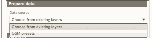
As mentioned earlier, this section defines which data source to use for the Reach Analysis.

Network

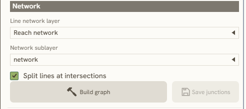
In the Line Network Layer, select a defined layer from your project. If you are using a .gpkg file that contains multiple sub-layers, you can access them using the Network Sublayer option.

B. Analysis Mode

Analysis Mode offers several operations. While each operation includes both Parameters and Interactive settings, the Closest to Set operation specifically requires a point layer.

In Parameters, you can configure the following settings:

Cutoff Distance: A predefined distance measured from your origin point.
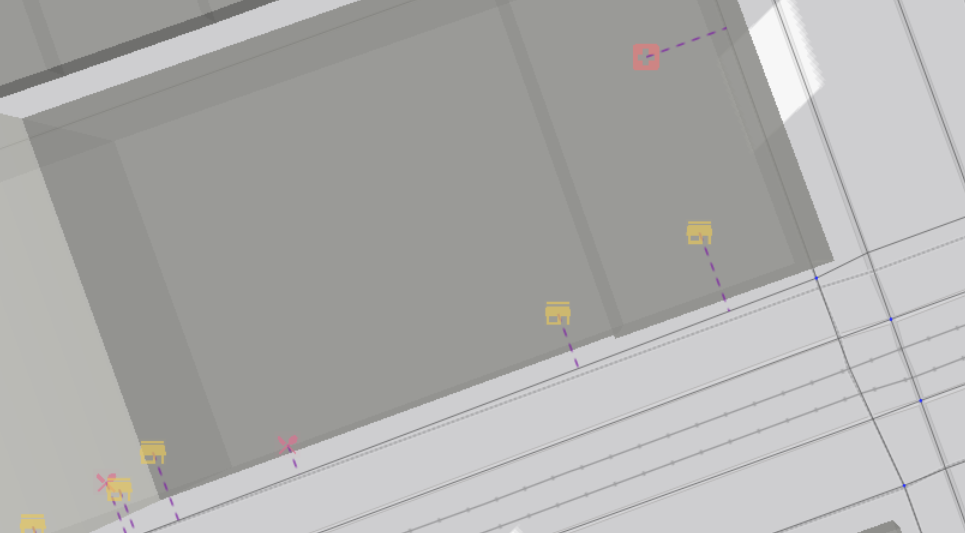
Entry Snap: A predefined distance used to snap both the origin and destination points to the nearest network (illustrated below).

In the Interactive section, you can select your origin input method using either Manual Draw or From Features:

Manual Draw: Interactively select points directly on the map.
From Features: Use an existing point layer from your project.

Coverage

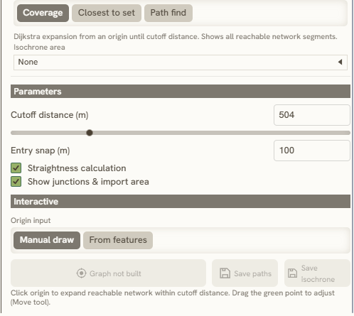
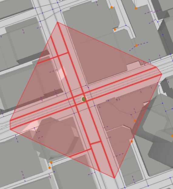
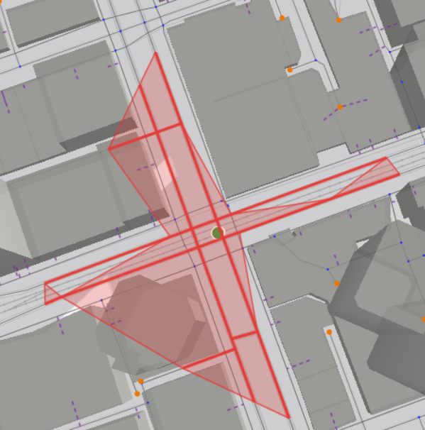
In coverage, there are several Isochrone method that can be used:

None	Isochrone by Convex	Isochrone by Concave Hull	Isochrone by Buffer

Missing attachment: Pasted image 20260729133941.png\

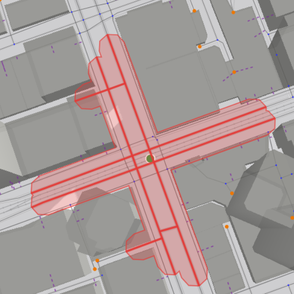
Closest to Set

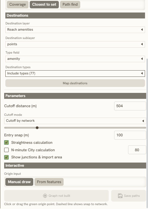
This operation analyzes each point treated as a destination, calculating Distance, Straightness, and Travel Time (N-minute) metrics relative to the origin point and its distance.

If you select the N-Minute City calculation, the Cutoff Distance automatically changes to 2000m.

Path Find

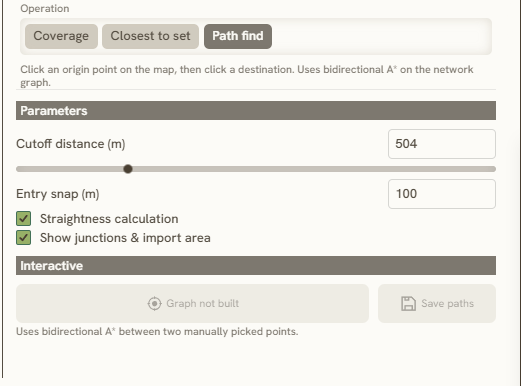
In Path Finding, you can analyze the shortest and most efficient route between your origin and destination points. This requires clicking the map twice: the first click sets the origin point, and the second click sets the destination point.

C. Result

As a result, two metrics will be displayed:

Highlighted: Displays metrics for the selected or hovered path.
Table: Displays overall metrics calculated from the analysis.